[ML] 2주차(1)

   요약

* 미분 공부가 필요할 것 같다. 확 와닿지 않는다.
* 이때까지의 진도가 모두의 딥러닝 부분에서 완전히 이해한 부분이 대부분이어서 어려움 없이 넘어갔었는데, 2주차부터는 새로운 내용도 많아지고 수학적 개념을 모두의 딥러닝보다 자세히 설명하고 넘어가서 복습이 필요할 것 같다.

   소제목

Multiple Features

Note: [7:25 - θ^T is a 1 by (n+1) matrix and not an (n+1) by 1 matrix]

Linear regression with multiple variables is also known as "multivariate linear regression".

We now introduce notation for equations where we can have any number of input variables.

The multivariable form of the hypothesis function accommodating these multiple features is as follows:

In order to develop intuition about this function, we can think about θ0 as the basic price of a house, θ1 as the price per square meter, θ2 as the price per floor, etc. x_1 will be the number of square meters in the house, x_2 the number of floors, etc.

Using the definition of matrix multiplication, our multivariable hypothesis function can be concisely represented as:

This is a vectorization of our hypothesis function for one training example; see the lessons on vectorization to learn more.

Remark: Note that for convenience reasons in this course we assume x_{0}^{(i)} =1 \text{ for } (i\in { 1,\dots, m } )x0(i)=1 for (i∈1,…,m). This allows us to do matrix operations with theta and x. Hence making the two vectors 'θ' and x^{(i)}match each other element-wise (that is, have the same number of elements: n+1).]

Gradient Descent For Multiple Variables

The gradient descent equation itself is generally the same form; we just have to repeat it for our 'n' features:

In other words:

The following image compares gradient descent with one variable to gradient descent with multiple variables:

Gradient Descent in Practice I - Feature Scaling

Note: [6:20 - The average size of a house is 1000 but 100 is accidentally written instead]

We can speed up gradient descent by having each of our input values in roughly the same range. This is because θ will descend quickly on small ranges and slowly on large ranges, and so will oscillate inefficiently down to the optimum when the variables are very uneven.

The way to prevent this is to modify the ranges of our input variables so that they are all roughly the same. Ideally:

These aren't exact requirements; we are only trying to speed things up. The goal is to get all input variables into roughly one of these ranges, give or take a few.

Two techniques to help with this are feature scaling and mean normalization. Feature scaling involves dividing the input values by the range (i.e. the maximum value minus the minimum value) of the input variable, resulting in a new range of just 1. Mean normalization involves subtracting the average value for an input variable from the values for that input variable resulting in a new average value for the input variable of just zero. To implement both of these techniques, adjust your input values as shown in this formula:

Where μ_i is the average of all the values for feature (i) and s_i is the range of values (max - min), or s_i is the standard deviation.

Note that dividing by the range, or dividing by the standard deviation, give different results. The quizzes in this course use range - the programming exercises use standard deviation.

For example, if x_i represents housing prices with a range of 100 to 2000 and a mean value of 1000, then,

Gradient Descent in Practice II - Learning Rate

Note: [5:20 - the x -axis label in the right graph should be θ rather than No. of iterations ]

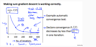
Debugging gradient descent. Make a plot with number of iterations on the x-axis. Now plot the cost function, J(θ) over the number of iterations of gradient descent. If J(θ) ever increases, then you probably need to decrease α.

Automatic convergence test. Declare convergence if J(θ) decreases by less than E in one iteration, where E is some small value such as 10^(−3). However in practice it's difficult to choose this threshold value.

It has been proven that if learning rate α is sufficiently small, then J(θ) will decrease on every iteration.

To summarize:

If α is too small: slow convergence.

If α is too large: may not decrease on every iteration and thus may not converge.

Features and Polynomial Regression

We can improve our features and the form of our hypothesis function in a couple different ways.

We can combine multiple features into one. For example, we can combine x_1 and x_2 into a new feature x_3 by talking x_1*x_2.

Polynomial Regression
Our hypothesis function need not be linear (a straight line) if that does not fit the data well.

We can change the behavior or curve of our hypothesis function by making it a quadratic, cubic or square root function (or any other form).

For example, if our hypothesis function is h_θ(x) = θ0 + θ1*x_1 then we can create additional features based on x_1, to get the quadratic function hθ(x) = θ0 + θ1x_1 + θ2(x_2)^2 or the cubinc function hθ(x) = θ0 + θ1x_1 + θ2(x_2)^2 + θ3(x_3)^3

In the cubic version, we have created new features x_2 and x_3 where x_2=(x_1)^2 and x_3=(x_1)^3.

To make it a square root function, we could do:  hθ(x) = θ0 + θ1x_1 + θ2sqrt(x_1)

One important thing to keep in mind is, if you choose your features this way then feature scaling becomes very important.

eg. if x_1 has range 1 - 1000 then range of x_1^2 becomes 1 - 1000000 and that of x_1^3 becomes 1 - 1000000000